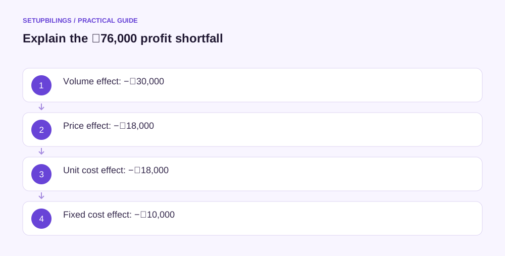
Learn from forecast differences by retaining the original forecast, reconciling actual results on the same basis and explaining the largest movements through measurable drivers. Separate volume, selling price, cost rate, spending and timing effects. Then decide whether the next forecast needs a new assumption, a corrective action or both.
A variance is information, not a complete performance judgement. A supplier price increase, an inaccurate estimate and unapproved rework can all raise costs, but they require different responses. The review should identify causes with evidence rather than treating every adverse figure as avoidable failure.
Preserve the forecast that existed beforehand
Consider an illustrative Surat industrial-label printer reviewing one month. The business retains the forecast approved before the month began, rather than comparing actuals with a version updated after most results were known. It identifies the data cut-off and whether late bills are estimated or final.
Use the same product groups, accounting period and cost boundaries. If a reporting category changed, prepare a bridge. Otherwise, a reclassification can look like a trading improvement or overspend.
ICAI's budget-control material connects responsibility, measurement, comparison and action. A practical review applies that sequence without allowing a long list of immaterial differences to distract from the result that needs attention.
Reconcile the profit difference
The printer forecast 1,000 units at ₹800, variable cost of ₹500 per unit and ₹2,00,000 fixed operating costs. Actual sales were 900 units at ₹780, variable cost ₹520 per unit and fixed costs ₹2,10,000.
| Illustrative monthly measure | Forecast | Actual |
|---|---|---|
| Units sold | 1,000 | 900 |
| Net selling price | ₹800 | ₹780 |
| Variable cost per unit | ₹500 | ₹520 |
| Sales | ₹8,00,000 | ₹7,02,000 |
| Variable costs | ₹5,00,000 | ₹4,68,000 |
| Contribution | ₹3,00,000 | ₹2,34,000 |
| Fixed operating costs | ₹2,00,000 | ₹2,10,000 |
| Operating profit | ₹1,00,000 | ₹24,000 |
Profit is ₹76,000 below forecast. Actual variable spending is lower in total, but that is not automatically favourable: fewer units were sold while variable cost per unit increased. The driver view prevents that misleading conclusion.
Explain the bridge through four drivers
First, 100 fewer units at the forecast ₹300 contribution reduce profit by ₹30,000. Second, the ₹20 price reduction across 900 actual units reduces it by ₹18,000. Third, the ₹20 variable-cost increase across 900 units reduces it by another ₹18,000. Fourth, higher fixed costs reduce it by ₹10,000.
The four effects total ₹76,000 and reconcile forecast profit of ₹1,00,000 to actual ₹24,000. This bridge uses one clear calculation convention. More complex mix or cost interactions may need additional analysis, but the total must still reconcile.
Do not apply the price change to forecast quantity in one part and actual quantity elsewhere without explaining the interaction. Consistent conventions make the bridge easier to review and repeat.
Investigate the business cause behind each driver
The lower volume could reflect lost demand, delayed dispatch or insufficient stock. Price weakness could come from authorised discounts, product mix or credit notes. Higher unit cost could reflect supplier revisions, lower yield or a different specification.
Use order records, quotations, production data and customer correspondence to distinguish them. “Sales were weak” is not enough if the real problem was a production delay that prevented accepted orders from shipping.
Record whether the cause is temporary or likely to persist. A delayed order expected next month needs timing evidence. A lost customer should not automatically be pushed into a later forecast to preserve the annual target.
Review cash variance separately
Suppose collections were forecast at ₹6,00,000 but actual receipts were ₹5,20,000. The ₹80,000 shortfall is a cash variance and is not identical to the ₹98,000 sales-revenue difference. Receipts may relate to earlier invoices, advances or different settlement timing.
Build a collection bridge using the invoices expected to pay, actual amounts and revised dates. If a receipt moves to next month, include it once there. If the customer disputes it, record the issue and the action needed rather than repeatedly forecasting payment without new evidence.
Review payment misses similarly: unplanned purchases, earlier supplier settlement and omitted periodic commitments affect cash differently from operating expense recognition.
Choose a small number of changes
For each material recurring cause, assign an action owner and review date. Purchasing might update supplier rates before quotes; sales might revise discount authority; production might correct an unreliable yield assumption. Avoid a long action list without priority.
Change forecasting assumptions when evidence shows the previous estimate was wrong. Take operational action where management can improve the outcome. Sometimes both are needed: correcting the forecast does not itself solve the operating problem.
Use materiality without hiding repeated errors
Set a review threshold suited to the business's scale, but also look for small differences that recur in the same direction. A minor courier underestimate repeated across many orders can become significant over a year. The threshold should keep the meeting focused while allowing persistent patterns to change the underlying forecast assumption.
Measure whether the forecast improves
Track errors by driver and by forecast horizon. Near-term forecasts should usually have stronger evidence than distant estimates. A repeated pattern of optimistic collections or understated unit costs should be visible across several periods.
Keep the original budget, latest forecast and actual result distinct. The review succeeds when the numbers reconcile, the major causes are understood and the next decision changes for a clear reason. That turns forecast variance from a monthly explanation exercise into a practical way to improve planning and execution.